Examples

Examples from our paper are generated upon installation of the package and can be found here.

Contact-implicit trajectory optimization

For a system modeled with $Q$ contact points, the smooth dynamics, as well as impact and friction, are modeled at each timestep $t$ with the following constraints:

\[\begin{align*} f_t(q_{t-1}, q_t, q_{t+1}) + B_t(q_t) u_t + C_t(q_t)^T \lambda_t &= 0, \\ \phi(q_{t+1}) &\geq 0, \\ \gamma_t \circ \phi_t(q_{t+1}) &= 0, \\ \beta_t^{(i)} \circ \eta_t^{(i)} &= 0, \quad i = 1, \dots, Q, \\ v^{(i)}(q_t, q_{t+1}) - {\eta_t}_{(2:3)}^{(i)} &= 0, \quad i = 1, \dots, Q, \\ {\beta_t}_{(1)}^{(i)} - \mu^{(i)} \gamma_t^{(i)} &= 0, \quad i = 1, \dots, Q, \\ \gamma_t, \phi_t(q_{t+1}) & \geq 0, \\ \beta_t^{(i)}, \eta_t^{(i)} &\in \mathcal{Q}^3, \quad i = 1, \dots, Q, \end{align*}\]

with configurations $q_t \in \mathbf{R}^{n_q}$, smooth discrete-time dynamics $f_t : \mathbf{R}^{n_q} \times \mathbf{R}^{n_q} \rightarrow \mathbf{R}^{n_q}$, input Jacobian $B_t : \mathbf{R}^{n_q} \rightarrow \mathbf{R}^{n_q \times m}$, contact Jacobian $C_t : \mathbf{R}^{n_q} \rightarrow \mathbf{R}^{3P \times n_q}$, contact impulses $\lambda_t \in \mathbf{R}^{3Q}$, signed distance $\phi_t : \mathbf{R}^{n_q} \rightarrow \mathbf{R}^P$, impact impulses $\gamma_t \in \mathbf{R}^P$, friction primals and duals $\beta_t, \eta_t \in \mathbf{R}^3$, contact-point tangential velocity $v : \mathbf{R}^{n_q} \times \mathbf{R}^{n_q} \rightarrow \mathbf{R}^2$, and friction coefficient $\mu \in \mathbf{R}_+$, where $\lambda = (\beta_{(2:3)}, \gamma)$. For additional details, see: [1] [2]

We utilize this formulation to optimize motions for:

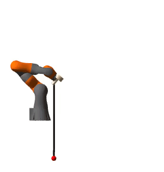
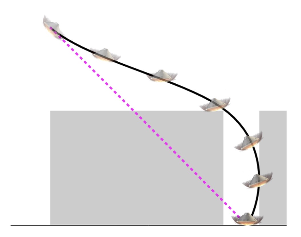
ball-in-cup

bunny hop

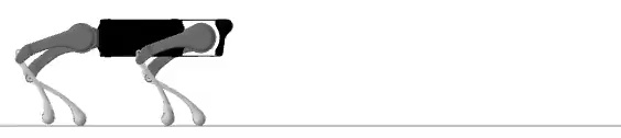
quadruped gait

drifting

State-triggered constraints

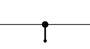
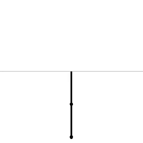
A trigger condition $\Gamma:\mathbf{R}^{n} \rightarrow \mathbf{R}$ encodes the logic: $\Gamma(x) > 0 \implies h(x) \geq 0$, that a constraint is enforced only when the trigger is satisfied. Such state-triggered constraints are utilized within various aerospace applications and commonly utilize a non-smooth formulation (left):

\[\begin{equation*} \text{min}(0, -\Gamma(x)) \cdot h(x) \leq 0 \quad \rightarrow \quad \begin{align*} \Gamma_+ - \Gamma_- &= \Gamma(x)\\ h_+ - h_- &= h(x) \\ \Gamma_+ \cdot h_- &= 0 \\ \Gamma_+, \Gamma_-, h_+, h_- & \geq 0. \end{align*} \end{equation*}\]

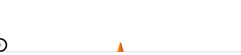
With CALIPSO, we employ an equivalent complementarity formulation (right) in order to land a rocket while avoiding keep-out zones.

Model-predictive control auto-tuning

A feedback policy is utilized to control underactuated robotic systems by tracking a reference $\bar{X}_{1:T}, \bar{U}_{1:T-1}$. The model-predictive control policy,

\[\begin{align*} \pi(\hat{X}; \theta) = U^*_1 = \underset{X_{1:H}, \phantom{\,} U_{1:H-1}}{\text{arg min }} & (X_H - \bar{X}_{[t + H]})^T P(\theta) (X_H - \bar{X}_{[t + H]}) + \sum \limits_{\tau = 1}^{H-1} (X_\tau - \bar{X}_{[t + \tau]})^T Q(\theta) (X_\tau - \bar{X}_{[t + \tau]}) + (U_\tau - \bar{U}_{[t + \tau]})^T R(\theta) (U_\tau - \bar{U}_{[t + \tau]}) \\ \text{subject to } & F_{\tau}(X_{\tau}, U_{\tau}) = X_{\tau+1}, \quad \tau = 1,\dots,H-1, \\ & X_1 = \hat{X}, \phantom{\, _{t+1}} \\ \end{align*}\]

computes controls by solving an optimization problem with horizon $H$ using CALIPSO and applying the first control to the system. Auto-tuning is performed to modify the weights in the policy's objective using gradient descent to minimize a metric that aims to minimize the difference between forward rollouts of the actual system and the reference trajectory.

cart-pole

(open-loop)

(untuned)

(MPC tuned)

acrobot

(open-loop)

(untuned)

(MPC tuned)